
One of the most basic tasks you need to perform when tuning SQL statements is determining the causes of the performance problem, and to do that, you will most likely need to analyze the execution plan of the problematic statement.
In this article, I cover the basics of execution plans, with the goal of helping people new to SQL tuning understand what they are and how they can be used as part of an SQL tuning process.
What is an Execution Plan?
You can think of an execution plan as the combination of steps used by the database to execute an SQL statement. In an execution plan, you can see the list of steps the database will have to perform to execute the statement, along with the cost associated with each step, which is very useful because you can see which of the steps are using more resources, and thus, probably taking more time to complete.
How do I Display an Execution Plan?
The method used to display an execution plan and the way it will be displayed may vary depending on the tool you are using.
If you are using SQL*Plus, you can set the AUTOTRACE system variable to ON or TRACEONLY, like this:
SET AUTOTRACE TRACEONLY;
This will make SQL*Plus display the execution plan for the query you are running.
You can also do something like this:
EXPLAIN PLAN FOR
[your query];
And then:
SELECT *
FROM TABLE(DBMS_XPLAN.DISPLAY());
If you are using SQL Developer, which is the tool I currently use, you can simply press the F10 key (for explain plan) or F6 (for autotrace), or simply click the appropriate button in the worksheet toolbar:
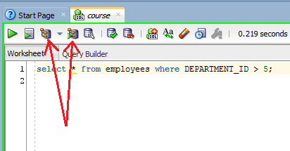
Explain Plan and Autotrace buttons in SQL Developer
Explain Plan vs. Autotrace
Explain plan and autotrace produce similar results (both of them display an execution plan), but there are two key differences:
- The plan displayed by explain plan is the one that the database “thinks” or predicts it will use to run the query, whereas the plan displayed by autotrace is the plan that was actually used to run the query (at least that is the case when using autotrace in SQL Developer), and that is why in some cases you can get different plans for the same query depending on how you generate it.
- Besides the execution plan, autotrace displays some statistics or metrics about each of the steps performed to execute the query, which can be very useful in investigating performance issues.
That is why I prefer to use autotrace over explain plan in most situations. The only disadvantage of autotrace could be that it actually executes the statement, so if you want to see the execution plan for a query that takes a very long time to run, you would get it much faster by using explain plan.
The documentation says that to use the autotrace utility you need the SELECT_CATALOG_ROLE and SELECT ANY DICTIONARY privileges, but as far as I can tell, you actually only need SELECT_CATALOG_ROLE.
The Optimizer
The software or process in the database that is in charge of generating execution plans for every statement that needs to be executed is called “The Optimizer“. It usually generates more than one execution plan for every statement, and then, it tries to estimate which of the candidate plans would be more efficient.
To make this estimation, the optimizer looks at the many statistics the database collects about the database and the objects involved in the statement, such as the number of rows in the involved tables, the average size of rows, the number of distinct values in columns, I/O and CPU usage, etc, etc, and then it assigns a cost to each of the steps in the plan. This cost is a number that represents the estimated resource usage for each step, and it is not measured in seconds, or CPU time, or memory bytes needed, or anything else. It is just a number or an internal unit that is used to be able to compare different plans.
After the optimizer has estimated the cost for each of the candidate plans, it chooses the one with the lowest total cost, which is why it is also called the “cost-based” optimizer. So, for example, if there are 2 execution plans for a query, and one of them includes 15 steps with a total cost of 30, and there is another candidate plan with only 5 steps but a total cost of 40, then the first one is used, because it has the lowest cost.
Besides estimating costs and choosing the best execution plan for each statement, the optimizer can also decide to “transform” a query into a different statement that would produce the same results in a more efficient manner, but I’m not going to talk about that component of the optimizer here, to keep this article as short and understandable as possible.
Types of Operations in an Execution Plan
The operations you see in an execution plan can be categorized into 2 main types: Those that access or retrieve data, and those that manipulate data retrieved by another operation.
Here is an image of how SQL Developer displays execution plans:
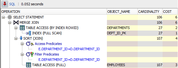
Tabular Execution Plan
Although we see the plan in a tabular form, an execution plan is actually a tree, which is traversed from top-down, left-to-right to display it as we see it in the image.
Here is how this plan would look like if it was displayed as a tree:
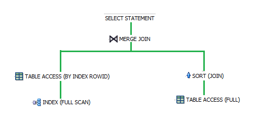
Tree-shaped Execution Plan
As you probably deducted from the images above, the operations are displayed in the opposite order of which they are performed. In the case of this tree, the data is read from the appropriate indexes and tables first (the leaves of the tree), and when both result sets are ready, they are joined together (the MERGE JOIN operation). In the case of the tabular representation, the operations more deeply indented are the ones executed first.
From now on, I will only refer to the tabular representation of the plan, because that is how you will most likely see it.
The first line we see is the line that represents the whole statement being evaluated, so the cost we see associated with that line is the total cost for the execution of the statement.
In general, the cost displayed for each operation accounts for the sum of the costs of its children. In this example, as you can see from the tree image above, the TABLE ACCESS for the departments table and the SORT (JOIN) are the direct children of the MERGE JOIN, so, since the table access has a cost of 2 and the sort has a cost of 4, the merge join has a total cost of 6.
From the second line on, we see the operations that the database will perform to get the desired results. Every operation has an associated cost, so, those lines that don’t have a cost, are not operations but only informational details about the operation they are part of (in the case of the plan in the image, the access and filter predicates are just details about the SORT operation).
The operations that access or retrieve data are those that have an associated object name, which is the source from where they retrieve the data (a table, an index, etc). In the case of the plan in the image, the objects from which data is being retrieved are the DEPARTMENTS and EMPLOYEES tables, and the DEPT_ID_PK index.
The cardinality column shows an estimation of the number of rows that will come out of each of the operations, so in this case, the optimizer estimated that 107 rows would be retrieved from the employees table, and 27 from the departments table, to produce a final result set of 106 rows.
Operations that Retrieve Rows (Access Paths)
As I mentioned earlier, some operations retrieve rows from data sources, and in those cases, the object_name column shows the name of the data source, which can be a table, a view, etc. However, the optimizer might choose to use different techniques to retrieve the data depending on the information it has available from the database statistics. These different techniques that can be used to retrieve data are usually called access paths, and they are displayed in the operations column of the plan, usually enclosed in parenthesis.
Below is a list of the most common access paths with a small explanation of them (source). I will not cover them all because I don’t want to bore you 😉 . I’m sure that after reading the ones I include here you will have a very good understanding of what access paths are and how they can affect the performance of you queries.
Full Table Scan
A full table scan reads all rows from a table, and then filters out those rows that do not meet the selection criteria (if there is one). Contrary to what one could think, full table scans are not necessarily a bad thing. There are situations where a full table scan would be more efficient than retrieving the data using an index.
Table Access by Rowid
A rowid is an internal representation of the storage location of data. The rowid of a row specifies the data file and data block containing the row and the location of the row in that block. Locating a row by specifying its rowid is the fastest way to retrieve a single row because it specifies the exact location of the row in the database.
In most cases, the database accesses a table by rowid after a scan of one or more indexes.
Index Unique Scan
An index unique scan returns at most 1 rowid, and thus, after an index unique scan you will typically see a table access by rowid (if the desired data is not available in the index). Index unique scans can be used when a query predicate references all of the columns of a unique index, by using the equality operator.
Index Range Scan
An index range scan is an ordered scan of values, and it is typically used when a query predicate references some of the leading columns of an index, or when for any reason more than one value can be retrieved by using an index key. These predicates can include equality and non-equality operators (=, <. >, etc).
Index Full Scan
An index full scan reads the entire index in order, and can be used in several situations, including cases in which there is no predicate, but certain conditions would allow the index to be used to avoid a separate sorting operation.
Index Fast Full Scan
An index fast full scan reads the index blocks in unsorted order, as they exist on disk. This method is used when all of the columns the query needs to retrieve are in the index, so the optimizer uses the index instead of the table.
Index Join Scan
An index join scan is a hash join of multiple indexes that together return all columns requested by a query. The database does not need to access the table because all data is retrieved from the indexes.
Operations that Manipulate Data
As I mentioned before, besides the operations that retrieve data from the database, there are some other types of operations you may see in an execution plan, which do not retrieve data, but operate on data that was retrieved by some other operation. The most common operations in this group are sorts and joins.
Sorts
A sort operation is performed when the rows coming out of the step need to be returned in some specific order. This can be necessary to comply with the order requested by the query, or to return the rows in the order in which the next operation needs them to work as expected, for example, when the next operation is a sort merge join.
Joins
When you run a query that includes more than one table in the FROM clause the database needs to perform a join operation, and the job of the optimizer is to determine the order in which the data sources should be joined, and the best join method to use in order to produce the desired results in the most efficient way possible.
Both of these decisions are made based on the available statistics.
Here is a small explanation for the different join methods the optimizer can decide to use:
Nested Loops Joins
When this method is used, for each row in the first data set that matches the single-table predicates, the database retrieves all rows in the second data set that satisfy the join predicate. As the name implies, this method works as if you had 2 nested for loops in a procedural programming language, in which for each iteration of the outer loop the inner loop is traversed to find the rows that satisfy the join condition.
As you can imagine, this join method is not very efficient on large data sets, unless the rows in the inner data set can be accessed efficiently (through an index).
In general, nested loops joins work best on small tables with indexes on the join conditions.
Hash Joins
The database uses a hash join to join larger data sets. In summary, the optimizer creates a hash table (what is a hash table?) from one of the data sets (usually the smallest one) using the columns used in the join condition as the key, and then scans the other data set applying the same hash function to the columns in the join condition to see if it can find a matching row in the hash table built from the first data set.
You don’t really need to understand how a hash table works. In general, what you need to know is that this join method can be used when you have an equi-join, and that it can be very efficient when the smaller of the data sets can be put completely in memory.
On larger data sets, this join method can be much more efficient than a nested loop.
Sort Merge Joins
A sort merge join is a variation of a nested loops join. The main difference is that this method requires the 2 data sources to be ordered first, but the algorithm to find the matching rows is more efficient.
This method is usually selected when joining large amounts of data when the join uses an inequality condition, or when a hash join would not be able to put the hash table for one of the data sets completely in memory.
So, what do I do with all this Information?
Now that you have a basic understanding of what you see in an execution plan, let’s talk about the things you should pay attention to when investigating a performance issue.
One of the main reasons why you would want to look at the execution plan for a query is to try to figure out if the optimizer in fact chose the most efficient plan. This could not be the case if the query is not written correctly or if the statistics are not up-to-date, among other things.
For example, you might see that a full table scan is being performed on a large table when you know that accessing it through an existing index would be more efficient, or that 2 big tables are being joined by using a nested loop, when you think that a hash join would be more efficient.
One of the first things you could do to identify potential performance problems would be looking at the cost of each operation, and focusing your attention on the steps with the highest costs (but remember that the cost displayed for each step is the accumulated cost, or in other words, it includes the cost of its “child” operations).
Once you have identified the steps with the highest cost, you can review the access paths or joining methods used in those steps, to see if there is something you think should have done in a different way.
Also, since the metrics autotrace reports include the time used to complete each operation, you might want to identify the steps that took longer to complete as well, and review the methods used to execute them.
And, because autotrace also reports the number of rows actually returned or accessed by each step, you can compare that number to the number of rows the optimizer “predicted” for each step (the value in the cardinality column) to see how accurate the estimation was.
Why? Because if the decision to use a certain plan was based on incorrect estimations, then there is a good probability that the plan chosen is not really the most efficient one. For example, if the optimizer estimated that a table had only a few hundred rows, it might have decided to fully scan it, but if in reality it had several thousand rows, it could have been more efficient to access it through an index.
However, looking for the steps that took longer to complete and comparing estimates with actual rows returned by hand might not be an easy task when the explain plan you are analyzing is big.
Fortunately, recent versions of SQL Developer include a “HotSpot” utility, which performs these tasks for you. It will identify steps with significant differences between the cardinality and last_output_rows columns, and will also identify the steps where the most time was spent.
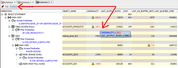
HotSpot feature in SQL Developer
This is a very useful feature that can save you time and effort.
There is also another very useful feature of SQL Developer, that allows you to compare two execution plans or autotrace outputs, so that you can easily spot the things the optimizer did different and how any change you made affected the execution plan selected.
To compare 2 plans you just need to pin the output of the first plan, then perform the changes you want to test in your query and get another execution plan. Once you have the 2 plans, you just need to right-click on the title of one of the plan panes and select the “compare with..” option as in this image:
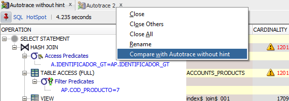
Execution plans comparison
This will give you a detailed report of the differences between the plans and the metrics gathered during the execution of the statements, which can be very useful to decide whether the changes you are testing produce the results you expected.
Okay, that’s it for this article. I hope that it has helped you at least a little bit to understand what execution plans are and what to look at when analyzing them.
Now you might want to know what you can do to fix the problems detected by analyzing an execution plan, but if I include that information here, this article would become a small book 😀 , so, that will be the topic for another post.
Please share your thoughts, doubts or suggestions in the discussion section below.
Happy tuning!
Subscribe to be informed about new posts, tips and more awesome things.